DataLoaders

Author

Marie-Hélène Burle

A critical part of deep learning is the loading of data to the model during the training loops.

DataLoaders handle the choice of which sample to load and in what order; they optimize the process in parallel by managing workers; they set several hyperparameters such as batch size and number of epochs.

In this section we explore DataLoaders with the Grain library [1].

Minimal necessary code from previous sections

base_dir = '<path-of-the-nabirds-dir>'

To be replaced by actual path: in our training cluster, the base_dir is at /project/def-sponsor00/nabirds:

base_dir = '/project/def-sponsor00/nabirds'

import os
import polars as pl
import imageio.v3 as iio
import grain.python as grain


metadata = pl.read_parquet('metadata.parquet')
metadata_train = metadata.filter(pl.col('is_training_img') == 1)
metadata_val = metadata.filter(pl.col('is_training_img') == 0)
cleaned_img_dir = os.path.join(base_dir, 'cleaned_images')


class NABirdsDataset:
    """NABirds dataset class."""
    def __init__(self, metadata, data_dir):
        self.metadata = metadata
        self.data_dir = data_dir

    def __len__(self):
        return len(self.metadata)

    def __getitem__(self, idx):
        path = os.path.join(self.data_dir, self.metadata.get_column('path')[idx])
        img = iio.imread(path)
        species_name = self.metadata.get_column('species_name')[idx]
        species_id = self.metadata.get_column('species_id')[idx]
        photographer = self.metadata.get_column('photographer')[idx]

        return {
            'img': img,
            'species_name': species_name,
            'species_id': species_id,
            'photographer': photographer,
        }


nabirds_train = NABirdsDataset(metadata_train, cleaned_img_dir)
nabirds_val = NABirdsDataset(metadata_val, cleaned_img_dir)

---------------------------------------------------------------------------
ModuleNotFoundError                       Traceback (most recent call last)
Cell In[2], line 3
      1 import os
      2 import polars as pl
----> 3 import imageio.v3 as iio
      4 import grain.python as grain
      5 
      6 

ModuleNotFoundError: No module named 'imageio'

Goal of DataLoaders

We can access elements of our Dataset class (as we did in the previous section) with:

for i, element in enumerate(nabirds_train):
    print(element['img'].shape)
    if i == 3:
        break

---------------------------------------------------------------------------
NameError                                 Traceback (most recent call last)
Cell In[3], line 1
----> 1 for i, element in enumerate(nabirds_train):
      2     print(element['img'].shape)
      3     if i == 3:
      4         break

NameError: name 'nabirds_train' is not defined

And we can return the next object by creating an iterator from an iterable dataset:

next(iter(nabirds_train))

---------------------------------------------------------------------------
NameError                                 Traceback (most recent call last)
Cell In[4], line 1
----> 1 next(iter(nabirds_train))

NameError: name 'nabirds_train' is not defined

We are getting all these 0 because we padded the images with black.

But all this is extremely limited.

DataLoaders feed data to the model during training. They handle batching, shuffling, sharding across machines, the number of epochs, etc. All things that would be very inconvenient to implement from scratch.

Grain DataLoaders

The JAX AI stack includes the Grain library [1] to create DataLoaders, but it can also be done using PyTorch, TensorFlow Datasets, Hugging Face Datasets, or any method you are used to. That’s the advantage of the modular philosophy that the stack relies on. Grain is extremely efficient and does not rely on a huge set of dependencies as PyTorch and TensorFlow do.

In Grain, a DataLoader requires 3 components:

A data source
Transforms
A sampler

Data source

We already have that: our data sources are our instances of Dataset class nabirds_train and nabirds_val for training and validation respectively.

Transformations

We need to split the data into batches. Batches can be defined with the grain.Batch method as a DataLoader transformation.

Let’s use batches of 32 with grain.Batch(batch_size=32).

How to choose the batch size?

The batch size is a crucial hyperparameter: it impacts your training speed, model stability, and final accuracy.

Default strategy

If you are unsure where to start, use a batch size of 32.

32 is small enough to provide a regularizing effect (helping the model generalize) but large enough to benefit from parallel processing on GPUs.

Standard values

Always use powers of 2 (32, 64, 128, 256) because GPUs and CPUs are optimized for binary operations, and this aligns memory allocation efficiently.

	Small batch size	Large batch size
Training speed	Slower: less efficient use of GPU	Faster: maximizes GPU throughput
Generalization	Better: the “noise” in the gradient helps the model escape sharp local minima	Worse: can lead to overfitting
Convergence	Noisy training curve: loss fluctuates	Smoother training curve: stable descent
Memory usage	Low: good for limited VRAM	High: risk of OOM

Tuning the batch size

Ceiling

Your maximum batch size is dictated by your GPU memory (VRAM).

If you hit an out of memory (OOM) error, you need to back down to the previous successful power of 2 (this is your hardware maximum).

Performance

Just because you can fit a batch size of 4096 doesn’t mean you should.

If training is stable but slow, double to 64, then double again to 128. You can increase the batch size to the hardware maximum to speed up epochs.

If the model overfits or diverges, try reducing the batch size. The “noisy” updates act like regularization, preventing the model from memorizing the data too perfectly.

Advanced techniques

Gradient accumulation:

If you need a batch size of 64 for stability but your GPU only fits 16, you can use gradient accumulation. You process 4 mini-batches of 16, accumulate the gradients, and update the weights once. This mathematically simulates a batch size of 64.

Dynamic batching:

Some advanced training regimes start with a small batch size to stabilize early training and increase it over time to speed up convergence (similar to learning rate decay).

Learning rate

If you change your batch size significantly, you should adjust your learning rate.

A rule that works well until you get to very large batch sizes is to double the learning rate when you double the batch size.

Samplers

There are 2 types of Grain samplers: sequential and index samplers.

Sequential sampler

Grain comes with a basic sequential sampler.

import grain.python as grain

nabirds_train_seqsampler = grain.SequentialSampler(
    num_records=4
)

for record_metadata in nabirds_train_seqsampler:
    print(record_metadata)

---------------------------------------------------------------------------
ModuleNotFoundError                       Traceback (most recent call last)
Cell In[5], line 1
----> 1 import grain.python as grain
      2 
      3 nabirds_train_seqsampler = grain.SequentialSampler(
      4     num_records=4

ModuleNotFoundError: No module named 'grain'

Index sampler

Grain index sampler is the one you should use as it allows for global shuffling of the dataset, setting the number of epochs, etc.

nabirds_train_isampler = grain.IndexSampler(
    num_records=200,
    shuffle=True,
    seed=0
)

for i, record_metadata in enumerate(nabirds_train_isampler):
  print(record_metadata)
  if i == 3:
      break

---------------------------------------------------------------------------
NameError                                 Traceback (most recent call last)
Cell In[6], line 1
----> 1 nabirds_train_isampler = grain.IndexSampler(
      2     num_records=200,
      3     shuffle=True,
      4     seed=0

NameError: name 'grain' is not defined

Let’s experiment with DataLoaders

With sequential sampler

nabirds_train_dl = grain.DataLoader(
    data_source=nabirds_train,
    sampler=nabirds_train_seqsampler,
    worker_count=0
)

---------------------------------------------------------------------------
NameError                                 Traceback (most recent call last)
Cell In[7], line 1
----> 1 nabirds_train_dl = grain.DataLoader(
      2     data_source=nabirds_train,
      3     sampler=nabirds_train_seqsampler,
      4     worker_count=0

NameError: name 'grain' is not defined

We can plot images in this sequential DataLoader:

import matplotlib.pyplot as plt

fig = plt.figure(figsize=(7.2, 9))

for i, element in enumerate(nabirds_train_dl):
    ax = plt.subplot(2, 2, i + 1)
    plt.tight_layout()
    ax.set_title(
        f"""
        {element['species_name']}
        Picture by {element['photographer']}
        """,
        fontsize=9,
        linespacing=1.5
    )
    ax.axis('off')
    plt.imshow(element['img'])

plt.show()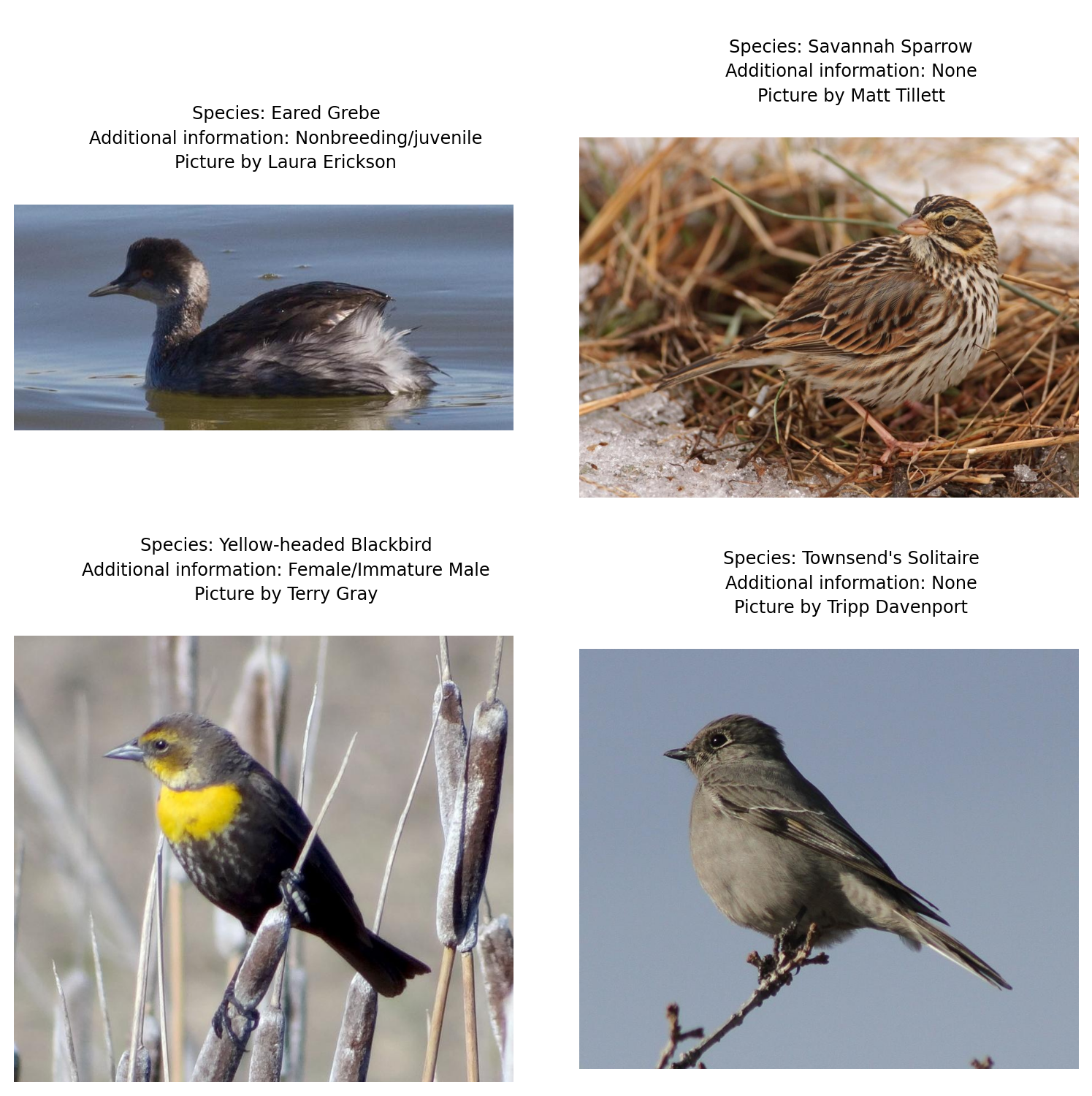

---------------------------------------------------------------------------
ModuleNotFoundError                       Traceback (most recent call last)
Cell In[8], line 1
----> 1 import matplotlib.pyplot as plt
      2 
      3 fig = plt.figure(figsize=(7.2, 9))
      4 

ModuleNotFoundError: No module named 'matplotlib'

Notice that, unlike last time we displayed some images, we aren’t looping through our Dataset (nabirds_train) anymore, but through our DataLoader (nabirds_train_dl).

Because we set the number of records to 4 in the sampler, we don’t have to break the loop.

With index sampler

nabirds_train_dl = grain.DataLoader(
    data_source=nabirds_train,
    sampler=nabirds_train_isampler,
    worker_count=0
)

---------------------------------------------------------------------------
NameError                                 Traceback (most recent call last)
Cell In[9], line 1
----> 1 nabirds_train_dl = grain.DataLoader(
      2     data_source=nabirds_train,
      3     sampler=nabirds_train_isampler,
      4     worker_count=0

NameError: name 'grain' is not defined

Let’s plot these as well:

fig = plt.figure(figsize=(7.2, 9))

for i, element in enumerate(nabirds_train_dl):
    ax = plt.subplot(2, 2, i + 1)
    plt.tight_layout()
    ax.set_title(
        f"""
        {element['species_name']}
        Picture by {element['photographer']}
        """,
        fontsize=9,
        linespacing=1.5
    )
    ax.axis('off')
    plt.imshow(element['img'])
    if i == 3:
        plt.show()
        break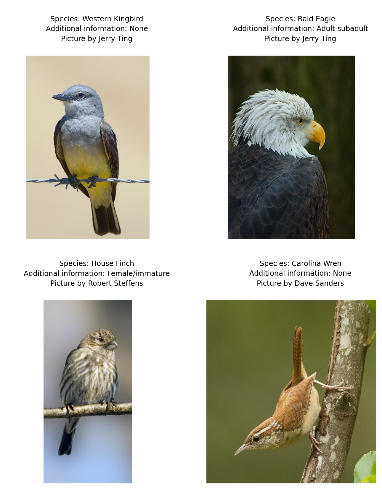

---------------------------------------------------------------------------
NameError                                 Traceback (most recent call last)
Cell In[10], line 1
----> 1 fig = plt.figure(figsize=(7.2, 9))
      2 
      3 for i, element in enumerate(nabirds_train_dl):
      4     ax = plt.subplot(2, 2, i + 1)

NameError: name 'plt' is not defined

Adding batch sizes

You can add the batch size in the operations argument of grain.DataLoader:

nabirds_train_dl = grain.DataLoader(
    data_source=nabirds_train,
    sampler=nabirds_train_isampler,
    worker_count=0,
    operations=[
        grain.Batch(batch_size=32)
    ]
)

---------------------------------------------------------------------------
NameError                                 Traceback (most recent call last)
Cell In[11], line 1
----> 1 nabirds_train_dl = grain.DataLoader(
      2     data_source=nabirds_train,
      3     sampler=nabirds_train_isampler,
      4     worker_count=0,

NameError: name 'grain' is not defined

Now we can access the next batch with:

next(iter(nabirds_train_dl))

---------------------------------------------------------------------------
NameError                                 Traceback (most recent call last)
Cell In[12], line 1
----> 1 next(iter(nabirds_train_dl))

NameError: name 'nabirds_train_dl' is not defined

References

Ritter M, Indyk I, Singh A, et al (2023) Grain - feeding JAX models