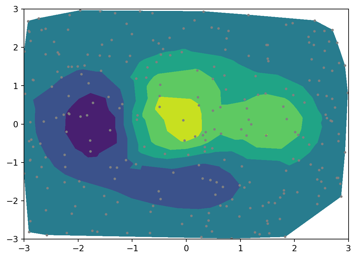
matplotlib is a very popular Python plotting library because it provides full control over the plots and produces graphs well-suited for publications. Many plot types can be created.
The downside of having full control is that it has a verbose imperative syntax. We will cover matplotlib in more details in the next course section.
Example
import matplotlib.pyplot as pltimport numpy as np# make data:np.random.seed(1)x = np.random.uniform(-3, 3, 256)y = np.random.uniform(-3, 3, 256)z = (1- x/2+ x**5+ y**3) * np.exp(-x**2- y**2)levels = np.linspace(z.min(), z.max(), 7)# plot:fig, ax = plt.subplots()ax.plot(x, y, 'o', markersize=2, color='grey')ax.tricontourf(x, y, z, levels=levels)ax.set(xlim=(-3, 3), ylim=(-3, 3))plt.show()
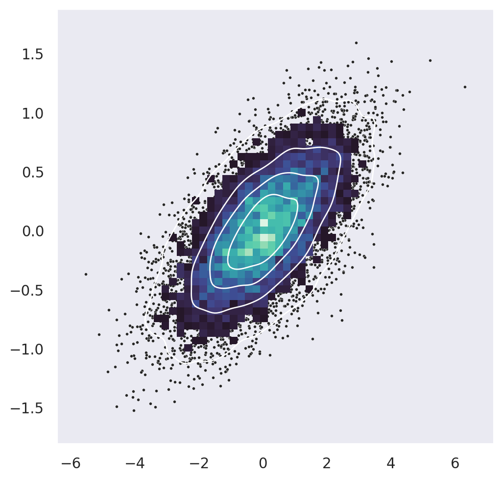
Seaborn is a higher level library built on top of matplotlib. This means that the options are more limited, but the declarative syntax is very easy, the defaults look great, and it has lots of statistical functionality, making it a perfect library for exploratory data analysis (EDA) on tabular data. We will also cover seaborn in more details later in this course.
Example
import numpy as npimport seaborn as snsimport matplotlib.pyplot as pltsns.set_theme(style="dark")# Simulate data from a bivariate Gaussiann =10000mean = [0, 0]cov = [(2, .4), (.4, .2)]rng = np.random.RandomState(0)x, y = rng.multivariate_normal(mean, cov, n).T# Draw a combo histogram and scatterplot with density contoursf, ax = plt.subplots(figsize=(6, 6))sns.scatterplot(x=x, y=y, s=5, color=".15")sns.histplot(x=x, y=y, bins=50, pthresh=.1, cmap="mako")sns.kdeplot(x=x, y=y, levels=5, color="w", linewidths=1);
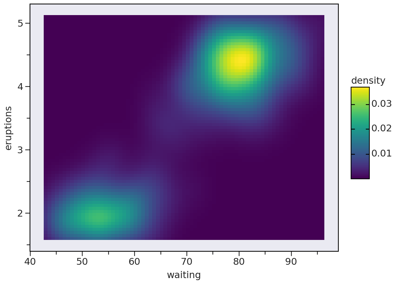
Gallery
For more examples, you can visit the seaborn gallery:
Bokeh creates interactive plots great for dashboards and web apps. It is more efficient than other libraries for streaming or interactions with large datasets. It does however have a fairly steep learning curve.
Example
from bokeh.models import LogColorMapperfrom bokeh.palettes import Viridis6 as palettefrom bokeh.plotting import output_notebook, figure, showfrom bokeh.sampledata.unemployment import data as unemploymentfrom bokeh.sampledata.us_counties import data as countiesoutput_notebook()palette =tuple(reversed(palette))counties = { code: county for code, county in counties.items() if county["state"] =="tx"}county_xs = [county["lons"] for county in counties.values()]county_ys = [county["lats"] for county in counties.values()]county_names = [county['name'] for county in counties.values()]county_rates = [unemployment[county_id] for county_id in counties]color_mapper = LogColorMapper(palette=palette)data=dict( x=county_xs, y=county_ys, name=county_names, rate=county_rates,)TOOLS ="pan,wheel_zoom,reset,hover,save"p = figure( title="Texas Unemployment, 2009", tools=TOOLS, x_axis_location=None, y_axis_location=None, tooltips=[ ("Name", "@name"), ("Unemployment rate", "@rate%"), ("(Long, Lat)", "($x, $y)"), ])p.grid.grid_line_color =Nonep.hover.point_policy ="follow_mouse"p.patches('x', 'y', source=data, fill_color={'field': 'rate', 'transform': color_mapper}, fill_alpha=0.7, line_color="white", line_width=0.5)show(p)
Plotly also creates interactive plots. It comes with two APIs: an older, lower-level, imperative one (Plotly Graph Objects) that allows for more control and a newer, higher-level, declarative one (Plotly Express) which is very easy to use. Static plots however are less sophisticated than with matplotlib and it is not as good as Bokeh for dashboard interactions.
We will have a quick look at plotly later in the course.
Example
You need to run the following to render plotly plots in Jupyter notebooks:
import plotly.io as piopio.renderers.default ='notebook'
Vega is a low-level, declarative, interactive visualization library for JSON.
On top of it was built Vega-Lite, a higher-level, simpler interactive JSON library.
Finally, Vega-Altair is a Python API built on top of Vega-Lite. It thus provides is a high-level, simple, declarative library for interactive plots. It is ideal for statistical visualization and EDA.
Example
import altair as altsource ="https://cdn.jsdelivr.net/npm/vega-datasets/data/us-employment.csv"predicate = alt.datum.nonfarm_change >0color = alt.when(predicate).then(alt.value("steelblue")).otherwise(alt.value("orange"))alt.Chart(source).mark_bar().encode( alt.X("month:T").title("Month"), alt.Y("nonfarm_change:Q").title("Month to month change in unemployment"), color=color, tooltip=[alt.Tooltip("nonfarm:Q", title="Unemployment that month")]).properties(width=650).interactive()
Gallery
For more examples, you can visit the Altair gallery: