Introduction to R for the humanities

Author

Marie-Hélène Burle

R is a free and open-source programming language for statistical computing, modelling, and graphics, with an unbeatable collection of statistical packages. It is extremely popular in some academic fields such as statistics, biology, bioinformatics, data mining, data analysis, and linguistics.

This introductory course does not assume any prior knowledge.

Running R

R being an interpreted language, it can be run non-interactively or interactively.

Running R non-interactively

If you write code in a text file (called a script), you can then execute it with:

Rscript my_script.R

The command to execute scripts is Rscript rather than R.
By convention, R scripts take the extension .R.

Running R interactively

There are several ways to run R interactively.

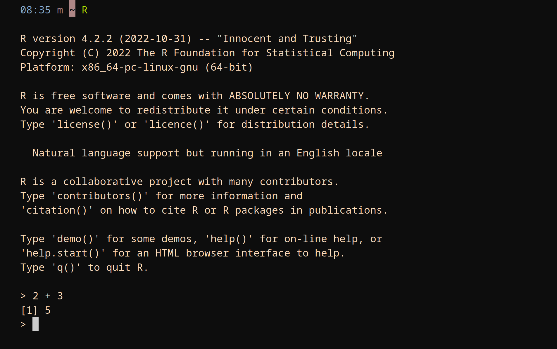
Directly in the console (the name for the R shell):

noshadow

In Jupyter with the R kernel (IRkernel package).
In another IDE (e.g. in Emacs with ESS).
In the RStudio IDE.

The RStudio IDE is popular and this is what we will use today. RStudio can can be run locally, but for this course, we will use an RStudio server.

Accessing our RStudio server

For this workshop, we will use a temporary RStudio server.

To access it, go to the website given during the workshop and sign in using the username and password you will be given (you can ignore the OTP entry).

This will take you to our JupyterHub. There, click on the “RStudio” button and our RStudio server will open in a new tab.

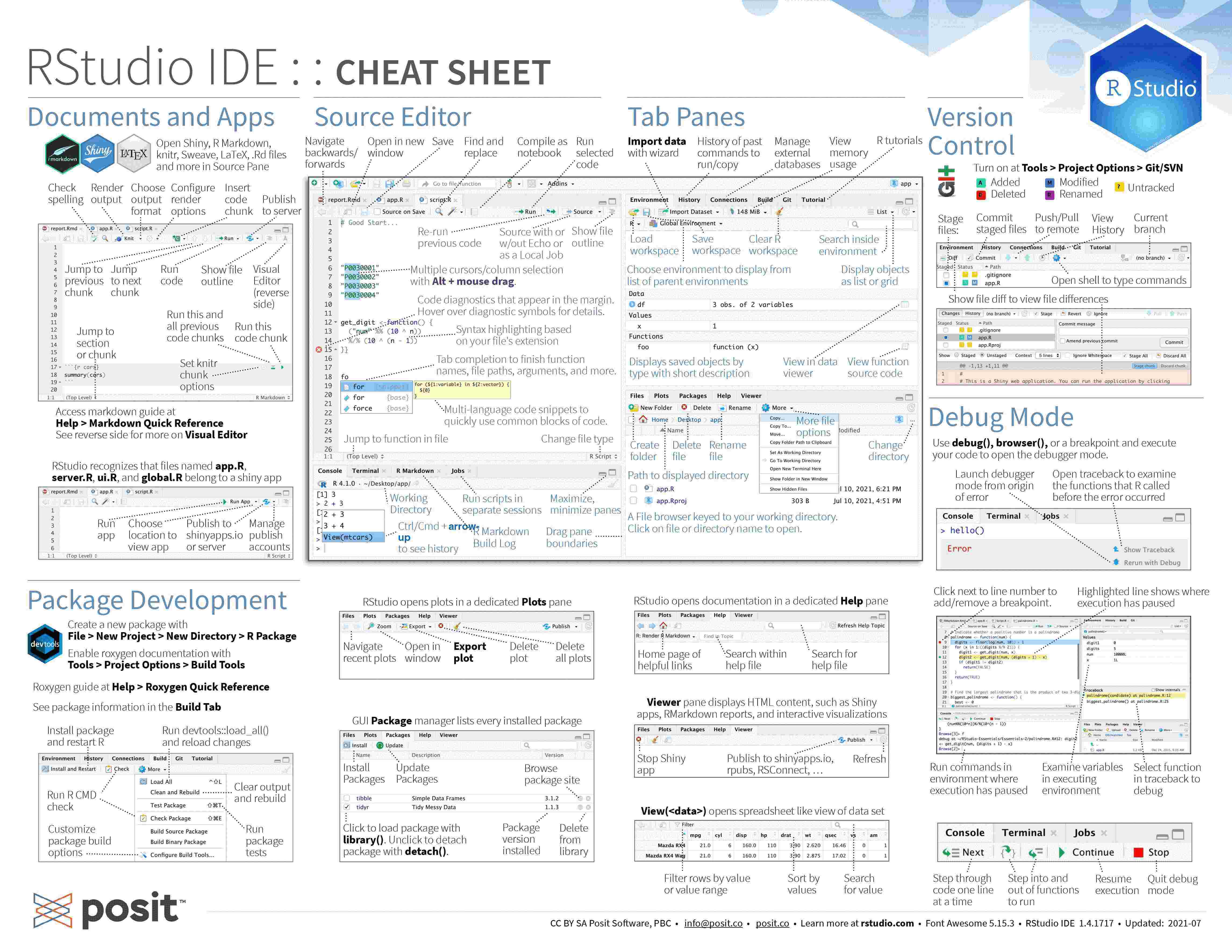
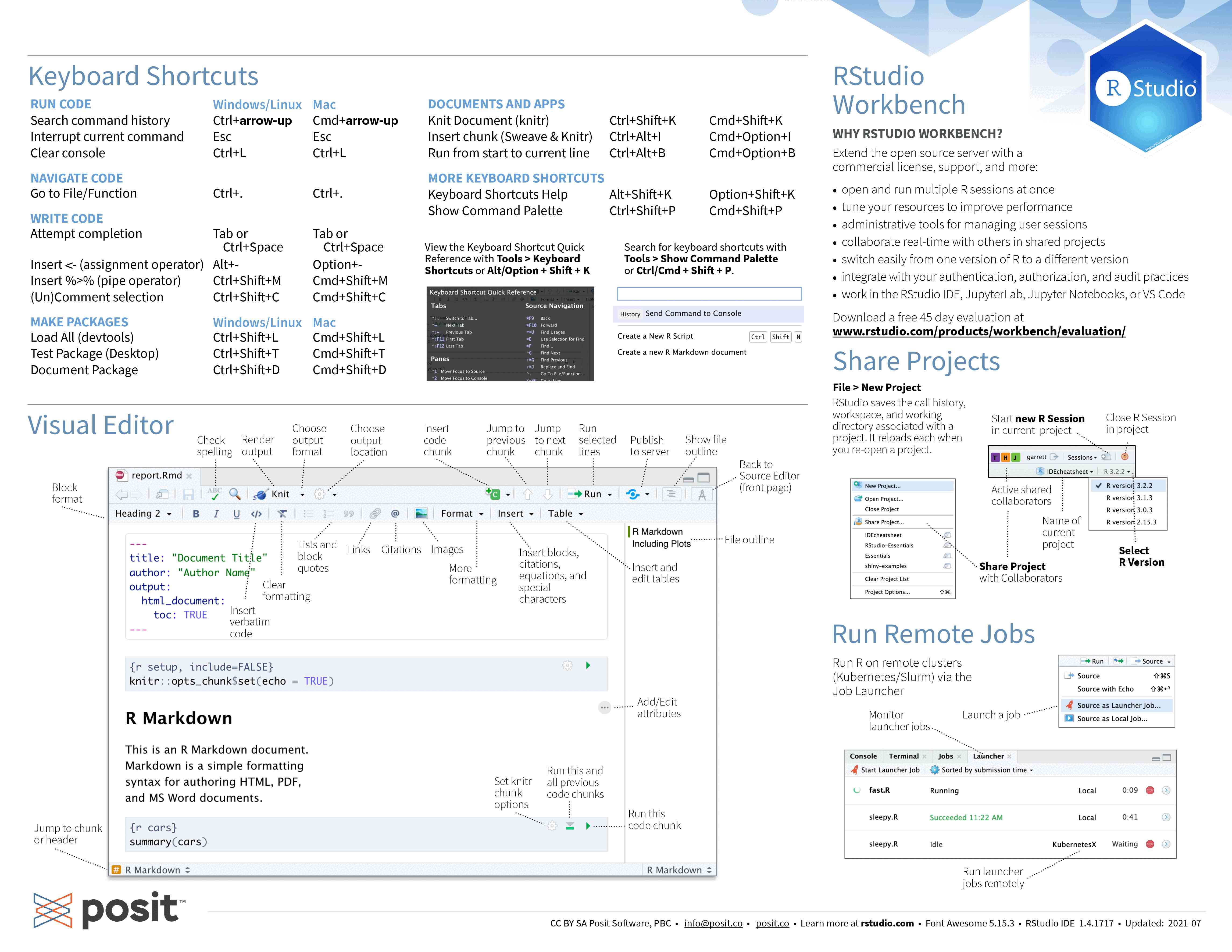
Using RStudio

For those unfamiliar with the RStudio IDE, you can download the following cheatsheet:

from Posit Cheatsheets

Help and documentation

For some general documentation on R, you can run:

help.start()

To get help on a function (e.g. sum), you can run:

help(sum)

Depending on your settings, this will open a documentation for sum in a pager or in your browser.

Basic syntax

Assignment

R can accept the equal sign (=) for assignments, but it is more idiomatic to use the assignment sign (<-) whenever you bind a name to a value and to use the equal sign everywhere else.

a <- 3

Once you have bound a name to a value, you can recall the value with that name:

a  # Note that you do not need to use a print() function in R

[1] 3

You can remove an object from the environment by deleting its name:

rm(a)
a

Error in eval(expr, envir, enclos): object 'a' not found

The garbage collector will take care of deleting the object itself from memory.

Comments

Anything to the left of # is a comment and is ignored by R:

# This is an inline comment

a <- 3  # This is also a comment

Data types and structures

Dimension	Homogeneous	Heterogeneous
1 d	Atomic vector	List
2 d	Matrix	Data frame
3 d	Array

Atomic vectors

vec <- c(2, 4, 1)
vec

[1] 2 4 1

typeof(vec)

[1] "double"

str(vec)

 num [1:3] 2 4 1

vec <- c(TRUE, TRUE, NA, FALSE)
vec

[1]  TRUE  TRUE    NA FALSE

typeof(vec)

[1] "logical"

str(vec)

 logi [1:4] TRUE TRUE NA FALSE

NA (“Not Available”) is a logical constant of length one. It is an indicator for a missing value.

Vectors are homogeneous, so all elements need to be of the same type.

If you use elements of different types, R will convert some of them to ensure that they become of the same type:

vec <- c("This is a string", 3, "test")
vec

[1] "This is a string" "3"                "test"

typeof(vec)

[1] "character"

str(vec)

 chr [1:3] "This is a string" "3" "test"

vec <- c(TRUE, 3, FALSE)
vec

[1] 1 3 0

typeof(vec)

[1] "double"

str(vec)

 num [1:3] 1 3 0

Data frames

Data frames contain tabular data. Under the hood, a data frame is a list of vectors.

dat <- data.frame(
  country = c("Canada", "USA", "Mexico"),
  var = c(2.9, 3.1, 4.5)
)
dat

  country var
1  Canada 2.9
2     USA 3.1
3  Mexico 4.5

typeof(dat)

[1] "list"

str(dat)

'data.frame':   3 obs. of  2 variables:
 $ country: chr  "Canada" "USA" "Mexico"
 $ var    : num  2.9 3.1 4.5

length(dat)

[1] 2

dim(dat)

[1] 3 2

Function definition

compare <- function(x, y) {
  x == y
}

We can now use our function:

compare(2, 3)

[1] FALSE

Note that the result of the last statement is printed automatically:

test <- function(x, y) {
  x
  y
}
test(2, 3)

[1] 3

If you want to return other results, you need to explicitly use the print() function:

test <- function(x, y) {
  print(x)
  y
}
test(2, 3)

[1] 2

[1] 3

Control flow

Conditionals

test_sign <- function(x) {
  if (x > 0) {
    "x is positif"
  } else if (x < 0) {
    "x is negatif"
  } else {
    "x is equal to zero"
  }
}

test_sign(3)

[1] "x is positif"

test_sign(-2)

[1] "x is negatif"

test_sign(0)

[1] "x is equal to zero"

Loops

for (i in 1:10) {
  print(i)
}

[1] 1
[1] 2
[1] 3
[1] 4
[1] 5
[1] 6
[1] 7
[1] 8
[1] 9
[1] 10

Notice that here we need to use the print() function.

Packages

Packages are a set of functions and/or data that add functionality to R.

Looking for packages

Package finder
Your peers and the literature

Package documentation

Managing R packages

R packages can be installed, updated, and removed from within R:

install.packages("package-name")
remove.packages("package-name")
update_packages()

Loading packages

To make a package available in an R session, you load it with the library() function.

Example:

library(readxl)

Alternatively, you can access a function from a package without loading it with the syntax: package::function().

Example:

readxl::read_excel("file.xlsx")

Publishing

You might have heard of R Markdown. It allows for the creation of dynamic publication-quality documents mixing code blocks, text, graphs…

The team which created R Markdown has now created an even better tool: Quarto. If you are interested in an introduction to this tool, you can have a look at our workshop or our webinar on Quarto.